
“Virtualise a non-linear sensor into a single linear function using the LInterp PROGMEM array generator
This tutorial shows you how to “Virtualise” a non-linear magnetic position sensor to produce an accurate linear position measurement from a single function call. It uses the LInterp array generator described in the ProjectHub tutorial “LInterp - A linear interpolation PROGMEM array generator” to produce a linear translation array for the sensor in program-space memory (PROGMEM). The resulting sensor measurement function uses no RAM storage. This scheme works on any Arduino board.
A simple magnetic position sensor
A Hall-effect magnetic flux sensor such as the Allegro Microsystems UGN3503 used in this tutorial makes an excellent contact-free short-range position sensor when used with a small rare-earth magnet positioned on the moving part being monitored. It is ideal where a position sensor must be fitted to existing equipment non-invasively (apart from a static magnetic field) or where a mechanical sensor would offer too much motive resistance. It also offers a high degree of position resolution, limited only by the chosen size of the translation array and the analog resolution of the Arduino board ADC.
The magnetic flux sensor comprises a small (about 0.5mm square) Hall-effect transistor coupled to an amplifier in a single three-terminal low-cost plastic transistor package. The Hall-effect transistor produces a current proportional to the magnetic flux density across it, which the amplifier scales to an output voltage between zero and its supply voltage (the UGN3503 is intended to operate from a 5V supply but may be used to a lower resolution with 3.3V). It may be employed in many geometries either as a near-static position sensor or a high-frequency (up to 20KHz) rotation encoder. Allegro provide a detailed design reference for the device. As a position encoder, the sensor requires a strong, small magnetic flux source such as a neodymium disc magnet to provide much physical range (millimeters) of measurement. However, the density of magnetic flux around a fixed magnet varies non-linearly with distance from its surface so the output voltage from the sensor will not vary linearly with its distance from the magnet. In fact, it is prohibitively difficult to calculate what the sensor should read for a given magnet and their mutual separation, and in practice the sensor-magnet response function is mapped across its intended range of use. This must be done with the sensor and magnet fitted in place within the device assembly being measured, so that the ambient magnetic field engendered by surrounding ferrous components forms part of the calibration. Accordingly, the magnetic sensor is best suited to permanent installation for (continuous or reference) position monitoring.
In the absence of any applied magnetic field (note: the Earth’s magnetic field is negligibly weak) the UGN3503 will output half its supply voltage, or 2.5V for a 5V nominal supply. A magnetic field of North (N) polarity applied to the front (logo side) of the device will drive the output towards zero volts and an applied field of South (S) polarity will drive the output towards the supply voltage. We can make the simplest position measurement by moving the magnet S pole across the sensor (see below) to produce a peaked output voltage / position relation. Note that, in the absence of any asymmetry imposed by the local magnetic environment, motion of the magnet toward the sensor from the left or right produces the same sensor output.
Mapping the sensor output
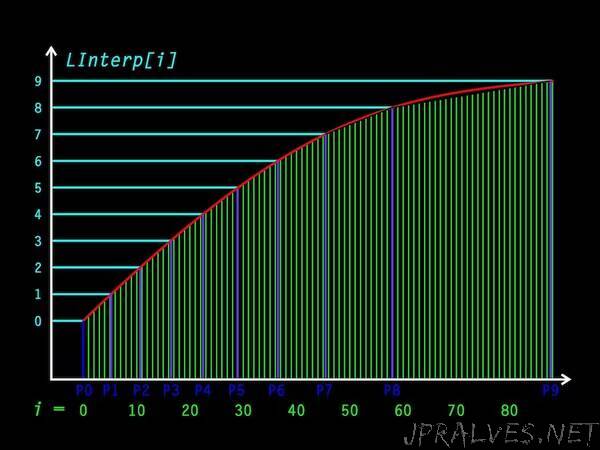
The number of mapping points required to achieve a given precision and accuracy for the measurement function is determined by the chosen size of the linear-transformation array and the resolution of the ADC. The latter forms a upper bound on the ultimate resolution possible fixed by hardware, but in most cases the memory dedicated to the array is the major constraint on measurement precision. The LInterp array generator greatly reduces this constraint by automatically placing the array in program-space (PROGMEM) memory, which is much larger than the microcontroller RAM. This is performed in compilation of the Arduino sketch so no run-time code is required. It also interpolates array values linearly between supplied mapping points, so a large array may be defined to achieve high translation precision from a smaller number of mapping points. Most importantly, the sensor output is mapped in uniformly-increasing (or decreasing) position increments for which the interpolator will automatically allocate more array elements in regions of rapid variation (response gradient, or slew rate) of the sensor output.
To select an array size and mapping point density, start by nominating a target function output resolution for the linear sensor virtualising function, in the desired output units, and calculate the required analog device output resolution (in millivolts) to achieve the desired function resolution at the magnet positions producing the smallest sensor-response gradients - either a magnet at maximum distance from the sensor, or a magnet directly under the sensor. Assuming the default Arduino-board ADC resolution of 10 bits or 1024 levels and an analog reference voltage (AREF) of 5.000V (and remembering that the ADC will only read up to AREF - 1 LSB) we obtain an intrinsic ADC resolution of (approx) 5mV for any device attached to an analog input.
For this example, we will adopt a single-magnet geometry in which the magnet is located on the edge of a 50mm-diameter metal disc which is rotated to bring the S-pole of magnet toward the sensor, for a minimum separation of 3mm. We choose an output scale of the disc orientation in degrees, which we can measure accurately using trigonometry by attaching a pointer to the disc and measuring how far its tip moves. We nominate a target angular resolution for the sensor output function of (say) 0.1 degree. By monitoring the output of the sensor using a voltmeter, we find that the difference between successive degree increments of the pointer drops to 20mV at a magnet position 12 degrees from the sensor. As 20mV equals about 4 ADC levels, we obtain a “device” angular resolution of only 0.25 degrees here, so an interpolation within 1-degree bounds will be out by at most 0.13 degrees (neglecting ADC error). If we take this position as both our resolution spec, range limit and zero position, then we can calculate the maximum size of the linear translation array corresponding to the highest possible resolution:
Sensor voltage at 0 degrees: 2.62V
Sensor voltage at 12 degrees: 4.21V
Required analog device resolution: 5mV
Maximum interpolation size at resolution limit: 4 ADC levels
Maximum array size = ( 4.21 - 2.62 ) / ( 4 * 0.005 ) = 80 elements (plus one element for the array interpolation upper bound)
Next, we decide how many mapping points we wish to measure based on the accuracy with which we can measure the pointer-divisions around our disc and an estimate of how much resolution we lose by using linear interpolations between mapping points for the translation array values. The latter constraint has greatest effect at the steepest regions of detector response, which in this case are seen on the voltmeter to occur for magnet positions between 5-6 degrees from the sensor, where the sensor gradient is about 500mV per degree. This figure corresponds to 25 array elements at our maximum interpolation size, but our chosen specification for angular resolution is satisfied by far fewer elements in this region. The over-allocation of array elements here is an unavoidable consequence of our (whole array) interpolation size specification being set to the device resolution limit at the extreme limit of the sensor’s response. If we manually interpolate a voltage prediction by taking the average of points 6 and 7 in the map, we obtain a predicted value of 3.33V; measuring the actual voltage at this position (6.5 degrees) on our disc, we get 3.29V or a worst-case interpolation error of 40mV. Accordingly, we can meet our angular resolution criterion everywhere by mapping the sensor at 1-degree intervals and interpolating linearly between them. [Advanced note: If we want extra mapping points in just one region of the map, so that the point spacing is irregular, then the whole map must be regularized. See the LInterp reference tutorial section “Irregularly-spacedordinate mapping sets” for details.]
Configuring the array generator
Taking a copy of the device-virtualiser outline header file LInDev.h from the LInterp reference tutorial and renaming it to LInMagSens.h, first we replace all occurrences of “DEV” in the header file with “MAG_SENS” to produce a unique set of definitions that won’t conflict with any in the sketch or its other header files. The sensor mapping-point voltage values we measured at 1-degree intervals of the magnet disc are now entered as definitions LI_P0 to LI_P12 in millivolts, and the remaining unused LI_Pn entries deleted. All the LI definitions are deleted by the array generator script after use so we need to keep copies of the array start and end positions (in millivolts) at the MAG_SENS_IN_MIN and MAG_SENS_IN_MAX labels (note the long-int type ‘L’ suffix to prevent integer arithmetic overflows in any user-supplied code). Next, we define our array output scaling at the MAG_SENS_OUT_ labels and define our interpolation size at MAG_SENS_INTERP. This completes the array definition._
Of vital importance to the correct translation of analog voltages with respect to our sensor map is the ACTUAL analog reference voltage, as measured at or applied to the Arduino board AREF pin. This is used by the ADC to scale input voltages to levels and must be supplied to the array generator at the ANALOG_RNG label, in millivolts. Do not assume the default 5000mV value shown, as the small on-board 5V regulator may be out by several hundred mV if it has been abused. Another common reference-voltage error is caused by assuming the USB-port 5V supply for AREF. Standard-compliant Arduino boards include a barrier diode in this supply, which drops the board operating voltage (and AREF) to about 4.65V. Errors caused by an incorrect ANALOG_RNG scale manifest as either missing or nonsense output values from the transform function for device output levels at or above the end of the transform array, whose sizes also changes according to ANALOG_RNG. Also remember that an external voltage reference used at the AREF pin requires the function call analogReference( EXTERNAL ); in setup() code or the MAG_SENS_Setup() device function prototype.
The LIndev.h header also includes prototype functions for device initialization, array interpolation and device access. These automatically refer to the customised value labels defined above and work without modification. Add to or alter these functions as required to isolate all device-specific code in the one header file and produce a single function call for a measurement from the underlying device. Unused functions will not be uploaded to the Arduino board. In our example the function MAG_SENS_ReadAvg() is wrapped in a macro called Position() which returns the current angle of the disc as a float value. The stub program LInMagSens.ino simply opens serial communications with the Arduino IDE serial monitor and returns a continuous sequence of calls to the Position() function.
The completed device virtualiser has used no RAM and ~700 bytes of code space memory, including ~350 bytes for the array. The used pgmspace.h library and analogRead() functions together occupy about 1.3K of code space memory, which does not add to further device definitions.”